The singular value decomposition

• The maximum gain problem and its relationship with norms
• The low-rank approximation of matrices
• The pseudo-inverse and least-squares problems
• The Schmidt decomposition: the singular value decomposition for linear operators
• Further reading

These are some introductory notes on the singular value decomposition. The singular value decomposition (SVD) is a particular matrix factorisation that has very useful properties. It is central to applications in data and model reduction because it solves the problem of finding the optimal approximation of a linear operator.

Theorem. Let \(M\) be a complex \(m \times n\) matrix. The decomposition \(M = U \Sigma V^*\) always exists, where \(U\) is an \(m \times m\) complex matrix, \(V\) is an \(n \times n\) complex matrix, \(\Sigma\) is a \(m \times n\) real matrix with diagonal elements \(\Sigma_{ii} = \sigma_i\) and \(\sigma_1 \geq \sigma_2 \geq \ldots\). The \(\sigma_i\) are called the singular values and the decomposition is called the singular value decomposition of \(M\). Matrices \(U\) and \(V\) are unitary, \(U U^* = U^* U = I_m\) and \(V V^* = V^* V = I_n\). \(\square\)

We can make the following observations. Since \(U\) and \(V\) are unitary, the rank of \(M\) is equal to the number of nonzero singular values. Notice that the inverse of a unitary matrix is its conjugate transpose.

The decomposition is only unique up to a constant complex multiplicative factor on each basis and up to the ordering of the singular values. That is, if \(U\Sigma V^*\) is a singular value decomposition, so is \((e^{i\theta} U) \Sigma (V^* e^{-i\theta})\). The columns of \(V\) and \(U\) that span the space corresponding to any exactly repeating singular values may be combined arbitrarily.

The structure of the singular value decomposition with \(n>m\) looks like this,

Truncation of \(\Sigma\) and \(V^*\) at the dotted lines give the reduced (or “compact”) SVD.

The maximum gain problem and its relationship with norms

It is helpful to think of \(M\) as an operator mapping a complex vector in the domain of \(M\) to another in the range of \(M\). The columns of \(V\), \(v_i\), provide a basis which spans the domain. The singular value decomposition of \(M\) can be written in terms of the vectors of \(U\) and \(V\),

Since \(V\) is unitary, \(v_i^* v_j = \delta_{ij}\), so applying \(M\) to \(v_j\) gives

Since \(V\) provides a basis for the domain of \(M\), any vector \(a\) in the domain of \(M\) can itself be expressed in terms of a weighted sum of columns of \(V\). That is, expressing \(a\) as

gives

We may then pose the question, what is the maximum amplitude of “output” for a given “input” amplitude? This is achieved with the input parallel to \(v_1\), with a gain of \(\sigma_1\). So,

is achieved with \(a / \|{a}\| = v_1\). Any other choice of \(a\) that is not parallel to \(v_1\) would achieve an inferior gain.

This is illustrated below for \(a\) of unit length. \(M\) maps a circle (ball) of unit radius to an ellipse (hyperellipse). The singular values are the major and minor axes of the ellipse.

We see the mapping of the unit circle (\(\|a\|=1\), left) to an ellipse (\(Ma\), centre) and mapping of \(Mv_1\) to \(\sigma_1 u_1\) (right). If we imagine the locus of points of \(a\) with unit length being drawn on a rubber sheet, the effect on \(M\) is to rotate and stretch the sheet. The amount of stretching in each direction is given by each singular value, and the directions by the singular vectors.

The low-rank approximation of matrices

For a non-square or rank-deficient square matrix, some of the singular values will be zero. In this case, the reduced SVD can be defined where the columns of \(U\) or \(V\) relating to the zero singular values, and the corresponding entries of \(\Sigma\), can be truncated with the decomposition remaining exact. In this case, though, \(U\) (or \(V\)) will not be unitary because the columns associated with the null space of \(M\) will have been truncated. This is illustrated in the earlier illustration, where the truncated columns of \(\Sigma\) and \(V\) are separated from the rest of the matrix by dotted lines.

Since these matrices often arise from numerical calculations, it is natural to ask what to do with singular values that are approximately zero within some defined threshold. If these are truncated, the decomposition forms an approximation to \(M\).

Where \(M\) is approximated by its SVD expansion truncated to order \(r\),

it can be seen that the approximation error is equal to the rest of the expansion (the “tail”),

and so is bounded,

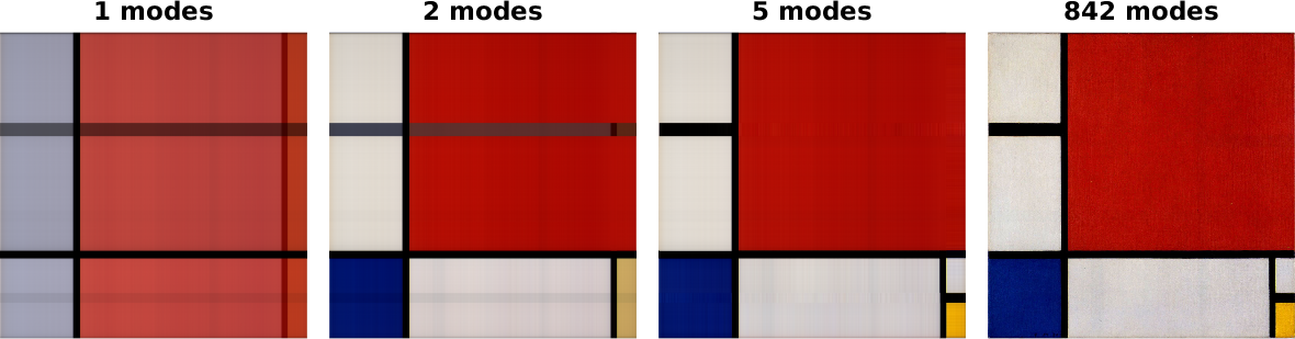
The effect of rank reduction can be seen by looking at the following Matlab code extract, which applies the SVD to images for various \(r\).

[U, S, V] = svd(img);
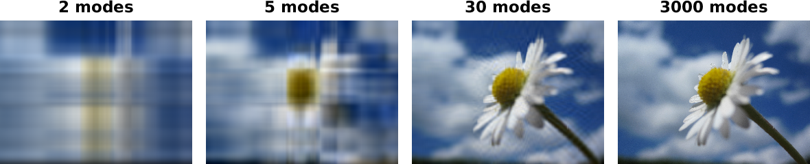
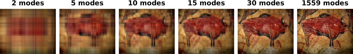
aprox_img = U(:,1:r) * S(1:r,1:r) * V(:,1:r)';

Here is the output for some sample images, showing progressively higher rank approximations of an image. The Mondrian picture is well-approximated by a very low-rank projection. The other image series, which have curves, require a high number of modes to capture the detail.

The pseudo-inverse and least-squares problems

I will briefly mention the pseudo-inverse here. A better and more detailed introduction (with proofs) is presented in Strang. The inverse of a matrix \(M\) in terms of its SVD is simply

Clearly \(\Sigma^{-1}\) only exists if \(M\) is full rank and square. Otherwise, we define the pseudo-inverse (or Moore-Penrose inverse) via the reduced SVD,

where \(\Sigma_r\) is the truncation of \(\Sigma\) to remove all zero singular values, so that \(\Sigma_r\) is invertible (the “reduced” SVD we saw earlier). \(M^+\) is a one-sided inverse (which side depends on whether \(m > n\); for example, if \(m > n\), then \(M M^+ = I_n\)).

Consider the under- or over-determined linear system of equations

A least squares solution \(x'\) that minimises \(\|{Mx - b}\|\) is given by

In the case where \(M\) does not have linearly independent columns, the solution \(x'\) (of all possible solutions) given by the pseudoinverse is the solution that has the minimum length. To see this, consider the \(n>m\) case illustrated earlier and denote the columns of \(V^*\) that were dropped in the reduced SVD as \(V^\perp\). Then \(M\) can be written as

The kernel of \(M\) is spanned by \(V^\perp\) so any component of \(x'\) in that space is “wasted” length.

The Schmidt decomposition: the singular value decomposition for linear operators

The matrix SVD has a direct analogy for linear operators on Hilbert spaces, called either the Schmidt decomposition or sometimes also the singular value decomposition, that is conceptually very similar to the matrix case. A good and detailed reference is Young. The following statement is equivalent to that in Curtain & Zwart. In the following, \(\left<\cdot, \cdot\right>_X\) represents the inner product on the space \(X\).

Theorem. If \(T : X \rightarrow Y\) is a compact (bounded, linear) operator, where \(X\) and \(Y\) are Hilbert spaces, then \(T\) has the following representation:

for some \(x \in X\) where the set \(\{\phi_i\}\) and the set \(\{\psi_i\}\) are the eigenvectors of \(T^*T\) and \(TT^*\) respectively, and \(\sigma_i \geq 0\) are the square roots of the eigenvalues. The \(\{\phi_i\}\) and \(\{\psi_i\}\) form an orthonormal basis for \(X\) and \(Y\) respectively (so \(\left<\psi_i, \psi_j\right>_Y = \delta_{ij}\) and so on). A pair \((\phi_i, \psi_i)\) is a Schmidt pair of \(T\) with an associated singular value \(\sigma_i\) and the decomposition is the Schmidt decomposition of \(T\). Further, \(T\) is bounded with norm \(\sigma_1\), so \(\|{Tx}\| \leq \sigma_1 \|{x}\|\). \(\square\)

Fortunately, many useful properties and much of the intuition arising from the simpler matrix SVD carry over to the operator case. The most obvious difference is that since \(X\) and \(Y\) are function spaces, there can be infinitely many singular values. Even then, \(T\) can still be approximated by a finite-rank operator with bounded error, in a manner analogous to the matrix case.

Further reading

The singular value decomposition is an extremely well established and widely used piece of mathematics. For the matrix case, the reader may find the presentations in Strang or Trefethen & Bau useful and insightful. The practical application in a control setting is well explained in Green & Limebeer. The operator case is thoroughly covered in Young and, in an infinite-dimensional linear systems setting, introduced in Curtain & Zwart.